How Many Productive Hours Make a Cobot Cell Pay?

The break-even answer in one equation

A cobot cell pays within the target period when its monthly value from good production equals or exceeds its monthly economic hurdle. The core calculation is: required productive hours per month = monthly recovery hurdle divided by net value per productive hour.

For a purchased cell, the monthly hurdle is the capital you intend to recover divided by the target payback months, plus fixed operating costs. For cobot rental, robot as a service, or monthly payment programs, use the recurring payment and other fixed costs instead of counting both a purchase price and financing payment.

Net value per productive hour is the labor expense genuinely avoided, overtime displaced, or contribution margin earned from additional good output, minus residual operator attendance and variable cell costs. The result is the minimum number of good-equivalent hours the cell must produce each month, not merely the time its controller is switched on.

What counts as a productive hour?

A productive hour is an hour of accepted output at the modeled rate. If the cell runs slowly, waits for parts, makes scrap, or requires an operator who could have completed the task manually, some of that clock hour has not created the value assumed in the business case.

NIST describes overall equipment effectiveness as fully productive time divided by planned production time. Its preferred calculation multiplies availability, performance, and quality. That framework is more useful for cobot break-even analysis than an uptime percentage because a cell can be technically available while starved, blocked, slowed, or producing rejected parts.

Keep three clocks in the model: assigned time, running time, and good-equivalent time. Assigned time has real demand behind it. Running time excludes planned and unplanned stops. Good-equivalent time further adjusts for lost speed and yield. Only the last clock belongs in the payback numerator.

How does the factory calendar become good hours?

Start with hours assigned to orders the cell can actually run. Subtract planned changeovers, sanitation, calibration, preventive maintenance, meetings, and any period when the cell has no eligible demand. Then apply measured factors for availability, material flow, speed, and first-pass quality.

A practical equation is: good-equivalent hours = assigned hours minus planned losses, multiplied by availability, flow factor, performance, and quality yield. The flow factor isolates starvation and downstream blockage. If your OEE system already assigns those losses to availability or performance, do not deduct them again.

This loss ledger should use cell data collected by reason code. Robot faults, gripper faults, empty infeed, full outfeed, operator unavailable, quality hold, planned setup, and preventive maintenance belong in separate buckets. A single downtime total conceals the operational owner and invites double counting.

• Assigned hours: scheduled time backed by qualified product demand
• Planned losses: changeover, cleaning, calibration, and planned maintenance
• Availability: remaining time after faults, recovery, and unplanned stops
• Flow factor: time retained after material starvation and downstream blockage
• Performance: actual rate divided by the validated good-production rate
• Quality: accepted units divided by total units produced

A worked utilization example

Consider an illustrative model expressed in normalized cost units, not market pricing. The cell must recover 1,200 units over 24 months and carries 10 units of fixed monthly expense. Each good-equivalent production hour creates 1.5 units of net value after variable costs and residual attendance.

The monthly hurdle is 1,200 divided by 24, plus 10, which equals 60 units. Required productive time is therefore 60 divided by 1.5, or 40 good-equivalent hours per month.

Now assume 100 assigned hours, with 10 hours of changeover and 5 hours of planned maintenance. Apply 90% availability, an 85% flow factor, 95% performance, and 98% quality. The cell produces 60.5 good-equivalent hours: 85 multiplied by 0.90, 0.85, 0.95, and 0.98.

That clears the 40-hour requirement. Yet the same loss profile means the cell needs 66.1 assigned hours to create those 40 productive hours. This distinction is the heart of utilization planning. A proposal claiming 40 hours of monthly use would miss payback if those were scheduled hours rather than good-equivalent hours.

How should operator attendance enter the model?

Collaborative does not mean unattended. A machine tending robot may still need racks replenished, doors cleared, offsets approved, gauges checked, and exceptions recovered. A palletizing cell may need labels, slip sheets, empty pallets, and finished loads removed.

Price that touch labor directly: attendance cost per productive hour = operator minutes required per productive hour divided by 60, multiplied by loaded labor cost. Include the supervisor, quality technician, material handler, and maintenance technician when their work is incremental. Do not claim an entire removed position when the job still consumes intermittent labor elsewhere.

The Bureau of Labor Statistics reported that private-industry compensation averaged $46.60 per employee hour in March 2026, including $32.60 in wages and $14.01 in benefits, with the total affected by rounding. That is not a shop-specific rate. It demonstrates why a wage-only input understates labor cost, so use payroll, benefit, overtime, and shift-premium data from the facility.

Attendance can also reduce productive time. If the cell stops whenever its shared operator is occupied, record that loss under operator unavailable. If the operator supports several machines without stopping the cobot, charge the labor fraction to the economics but leave productive hours intact.

Where do changeovers, maintenance, and scrap bite hardest?

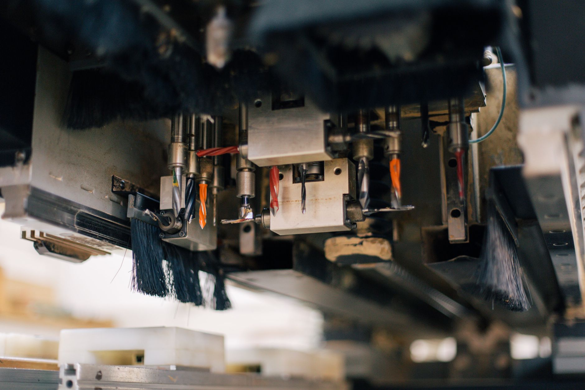
Changeovers consume capacity before the first accepted part. Count tool exchange, fixture movement, recipe loading, material presentation, safety checks, first-piece inspection, and the ramp to stable production. NIST notes that setup work commonly includes tool adjustment plus safety and quality checks, all of which affect flexible-line output.

The opportunity is measurable. One NIST Manufacturing Extension Partnership case began with an 8-hour, 20-minute changeover and 9,121 feet of employee travel. The improvement effort reduced changeover time by 70% and travel by 98%. Those figures are a documented case, not a universal expectation, but they show why setup observation can alter the payback more than a faster robot cycle.

Maintenance belongs in two places. Planned service reduces available production hours, while parts, consumables, remote support, and on-site labor affect cost. A maintenance included agreement may stabilize the expense line, but it does not erase service time from the capacity calculation. NIST's manufacturing maintenance analysis reported downtime equal to 13.3% of planned production time in its study data, reinforcing the need for a measured allowance rather than an assumption of perfect availability.

Scrap must be valued at the point where it occurs. Include consumed material, prior processing, disposal, rework, inspection, and lost bottleneck time. Apply quality yield to hours and subtract any incremental scrap cost from hourly value. Otherwise the model can count rejected production as a benefit while hiding its cost.

Can redeployment rescue a lightly loaded cell?

Redeployment can turn idle capacity into economic value, but only validated work counts. NIST identifies large changeover times and limited reusability as barriers to robotic agility. A portable base or reprogrammable arm does not by itself make a cell commercially fungible.

Model each product separately because rates, yields, attendance, tooling, and margins differ. The portfolio test is: sum of good-equivalent hours for each product multiplied by that product's net hourly value must exceed the monthly hurdle plus product-specific setup costs.

Demand calendars matter. Two products needed during the same shift cannot both claim the same cobot hours. Build a finite-capacity schedule that includes fixture storage, program control, risk-assessment updates, first-article approval, and movement between stations. Reserve capacity for schedule volatility instead of booking every theoretical minute.

Before including a second product in payback, run it through the commercial robot pilot program and document its accepted cycle rate, quality yield, setup duration, operator touch time, and demand window. Redeployment earns credit only after that evidence exists.

• Dedicated tooling and storage are available when the job is released
• Programs, recipes, and quality limits are revision controlled
• Material presentation works without chronic starvation
• Safety validation covers every station and end effector
• The production schedule contains nonoverlapping demand
• Changeover cost is smaller than the value of the added run

How should risk and financing change the threshold?

Run at least three cases: expected, downside, and demand loss. The downside case should lengthen changeovers, increase attendance, reduce yield, and include a realistic outage. The demand-loss case should remove a product or shift. A cell that pays only in the best case is not ready for approval.

Safety assumptions also affect rate and attendance. OSHA says robot applications require task-based risk assessment and that operators must be protected from hazards during automatic operation. Safeguarding, speed limits, separation monitoring, manual interventions, and restart procedures can therefore change the validated cycle, footprint, and staffing model.

Commercial structure should follow utilization confidence. Cobot rental for manufacturing, a collaborative robot arm rental, or a lease purchase program can align payments with uncertain demand, although contract terms still need careful modeling. A purchase can fit stable, heavily loaded work. Compare each path with the same productive-hour equation rather than treating no upfront capital as free capacity.

Service Robot Co. can build that comparison as an OEM-neutral, full-service commercial robot integrator for U.S. businesses. The team selects across manufacturers, then finances, deploys, integrates, trains, and services each unit through a nationwide U.S. engineer network. That one-vendor lifecycle helps keep cell design, economic assumptions, go-live support, and robot maintenance service plans tied to the same operating case.

What should be proven before approval?

Freeze the economic worksheet before the pilot so the success criteria cannot drift. Record the required productive hours, minimum good rate, maximum operator minutes, first-pass yield, changeover ceiling, availability floor, and monthly demand coverage. State who owns every source value and how often it will be refreshed.

During the pilot, capture several complete production runs and every loss reason. Include normal operators, representative materials, shift changes, replenishment, planned setups, quality checks, and fault recovery. A short demonstration with hand-selected parts validates motion, not monthly economics.

After go-live, compare the rolling productive-hour total with the break-even line each week. If the gap opens, the loss ledger points to the response: improve infeed reliability, shorten setup, correct quality drift, revise staffing, schedule another qualified product, or reconsider the target payback. Utilization becomes a managed operating variable, not a hopeful percentage in a capital request.